
Hopefully you will find enough information about how to set images in your blog here. This is an example of a post which includes a feature image specified in the front matter of the post. The feature image spans the full-width of the page, and is shown with the title on permalink pages:
CUSTOMER CHURN ANALYSIS
Import Library
# Library for data analysis
import numpy as np
import pandas as pd

# Library for visualization
import matplotlib.pyplot as plt
import seaborn as sns
%matplotlib inline

# Library for machine learning
from sklearn.model_selection import train_test_split, cross_val_score
from sklearn.metrics import confusion_matrix, classification_report
from sklearn.metrics import roc_curve, roc_auc_score
from sklearn.linear_model import LogisticRegression
import xgboost as xgb

# Setting parameter kernel
plt.rcParams['figure.figsize'] = [10,6]
sns.set_style('darkgrid')
Data Preparation
Import Raw Data
# Read file as dataframe
df = pd.read_csv('https://dqlab-dataset.s3-ap-southeast-1.amazonaws.com/data_retail.csv', sep = ';')
# Print first five rows
df.head()
| no | Row_Num | Customer_ID | Product | First_Transaction | Last_Transaction | Average_Transaction_Amount | Count_Transaction | |
|---|---|---|---|---|---|---|---|---|
| 0 | 1 | 1 | 29531 | Jaket | 1466304274396 | 1538718482608 | 1467681 | 22 |
| 1 | 2 | 2 | 29531 | Sepatu | 1406077331494 | 1545735761270 | 1269337 | 41 |
| 2 | 3 | 3 | 141526 | Tas | 1493349147000 | 1548322802000 | 310915 | 30 |
| 3 | 4 | 4 | 141526 | Jaket | 1493362372547 | 1547643603911 | 722632 | 27 |
| 4 | 5 | 5 | 37545 | Sepatu | 1429178498531 | 1542891221530 | 1775036 | 25 |
print('Info dataset:')
df.info()
Info dataset:
<class 'pandas.core.frame.DataFrame'>
RangeIndex: 100000 entries, 0 to 99999
Data columns (total 8 columns):
 #   Column                      Non-Null Count   Dtype
---  ------                      --------------   -----
 0   no                          100000 non-null  int64
 1   Row_Num                     100000 non-null  int64
 2   Customer_ID                 100000 non-null  int64
 3   Product                     100000 non-null  object
 4   First_Transaction           100000 non-null  int64
 5   Last_Transaction            100000 non-null  int64
 6   Average_Transaction_Amount  100000 non-null  int64
 7   Count_Transaction           100000 non-null  int64
dtypes: int64(7), object(1)
memory usage: 6.1+ MB
Data Wrangling
# Change format column First_Transaction and Last Transaction
df['First_Transaction'] = pd.to_datetime(df['First_Transaction']/1000, unit='s', origin='1970-01-01')
df['Last_Transaction'] = pd.to_datetime(df['Last_Transaction']/1000, unit='s', origin='1970-01-01')
# View new format
df[['First_Transaction','Last_Transaction']].head()
| First_Transaction | Last_Transaction | |
|---|---|---|
| 0 | 2016-06-19 02:44:34.395999908 | 2018-10-05 05:48:02.608000040 |
| 1 | 2014-07-23 01:02:11.493999958 | 2018-12-25 11:02:41.269999981 |
| 2 | 2017-04-28 03:12:27.000000000 | 2019-01-24 09:40:02.000000000 |
| 3 | 2017-04-28 06:52:52.546999931 | 2019-01-16 13:00:03.911000013 |
| 4 | 2015-04-16 10:01:38.530999899 | 2018-11-22 12:53:41.529999970 |
# Check Last Transaction update
print(max(df['Last_Transaction']))
2019-02-01 23:57:57.286000013
# Create new column is_Churn
df.loc[df['Last_Transaction'] <= '2018-08-01', 'is_Churn'] = True
df.loc[df['Last_Transaction'] > '2018-08-01', 'is_Churn'] = False
# Remove unnecessary columns
del df['no']
del df['Row_Num']
Clean Dataset
# View first five rows after cleaning data
df.head()
| Customer_ID | Product | First_Transaction | Last_Transaction | Average_Transaction_Amount | Count_Transaction | is_Churn | |
|---|---|---|---|---|---|---|---|
| 0 | 29531 | Jaket | 2016-06-19 02:44:34.395999908 | 2018-10-05 05:48:02.608000040 | 1467681 | 22 | False |
| 1 | 29531 | Sepatu | 2014-07-23 01:02:11.493999958 | 2018-12-25 11:02:41.269999981 | 1269337 | 41 | False |
| 2 | 141526 | Tas | 2017-04-28 03:12:27.000000000 | 2019-01-24 09:40:02.000000000 | 310915 | 30 | False |
| 3 | 141526 | Jaket | 2017-04-28 06:52:52.546999931 | 2019-01-16 13:00:03.911000013 | 722632 | 27 | False |
| 4 | 37545 | Sepatu | 2015-04-16 10:01:38.530999899 | 2018-11-22 12:53:41.529999970 | 1775036 | 25 | False |
# View info dataset
df.info()
<class 'pandas.core.frame.DataFrame'>
RangeIndex: 100000 entries, 0 to 99999
Data columns (total 7 columns):
 #   Column                      Non-Null Count   Dtype
---  ------                      --------------   -----
 0   Customer_ID                 100000 non-null  int64
 1   Product                     100000 non-null  object
 2   First_Transaction           100000 non-null  datetime64[ns]
 3   Last_Transaction            100000 non-null  datetime64[ns]
 4   Average_Transaction_Amount  100000 non-null  int64
 5   Count_Transaction           100000 non-null  int64
 6   is_Churn                    100000 non-null  object
dtypes: datetime64[ns](2), int64(3), object(2)
memory usage: 5.3+ MB
Data Visualization
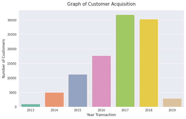
Customer Acquisition By Year
# Create new column Year First Transaction
df['Year_First_Transaction'] = df['First_Transaction'].dt.year
# Create new column Last Transaction
df['Year_Last_Transaction'] = df['Last_Transaction'].dt.year
# Grouping Number of Customers by Year
cust_by_year = df.groupby(['Year_First_Transaction'])['Customer_ID'].count()
cust_by_year
Year_First_Transaction
2013     1007
2014     4954
2015    11235
2016    17656
2017    31828
2018    30327
2019     2993
Name: Customer_ID, dtype: int64
# Plotting number of customers by year
sns.barplot(x = cust_by_year.index, y = cust_by_year, palette='Set2')
plt.title('Graph of Customer Acquisition', fontsize=15, pad=15)
plt.xlabel('Year Transaction', fontsize=12)
plt.ylabel('Number of Customers', fontsize=12)
Text(0, 0.5, 'Number of Customers')
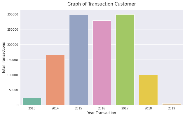
Transaction by Year
# Grouping total Count Transaction by Year
trans_by_year = df.groupby(['Year_First_Transaction'])['Count_Transaction'].sum()
trans_by_year
Year_First_Transaction
2013     23154
2014    165494
2015    297445
2016    278707
2017    299199
2018     99989
2019      5862
Name: Count_Transaction, dtype: int64
# Plotting total transactions by year
sns.barplot(x = trans_by_year.index, y = trans_by_year, palette='Set2')
plt.title('Graph of Transaction Customer', fontsize=15, pad=15)
plt.xlabel('Year Transaction', fontsize=12)
plt.ylabel('Total Transactions', fontsize=12)
Text(0, 0.5, 'Total Transactions')
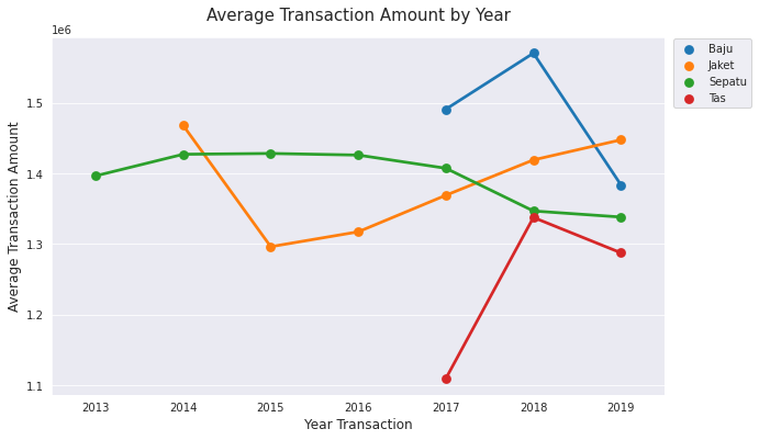
Average Transaction Amount by Year
# Grouping Average Transaction Amount by Product and Year
avg_trans_amount = df.groupby(['Product', 'Year_First_Transaction'])['Average_Transaction_Amount'].mean().reset_index()
avg_trans_amount
| Product | Year_First_Transaction | Average_Transaction_Amount | |
|---|---|---|---|
| 0 | Baju | 2017 | 1.490890e+06 |
| 1 | Baju | 2018 | 1.570201e+06 |
| 2 | Baju | 2019 | 1.383645e+06 |
| 3 | Jaket | 2014 | 1.467937e+06 |
| 4 | Jaket | 2015 | 1.296265e+06 |
| 5 | Jaket | 2016 | 1.317344e+06 |
| 6 | Jaket | 2017 | 1.369034e+06 |
| 7 | Jaket | 2018 | 1.419074e+06 |
| 8 | Jaket | 2019 | 1.447536e+06 |
| 9 | Sepatu | 2013 | 1.396499e+06 |
| 10 | Sepatu | 2014 | 1.427063e+06 |
| 11 | Sepatu | 2015 | 1.428235e+06 |
| 12 | Sepatu | 2016 | 1.425938e+06 |
| 13 | Sepatu | 2017 | 1.407275e+06 |
| 14 | Sepatu | 2018 | 1.346824e+06 |
| 15 | Sepatu | 2019 | 1.338180e+06 |
| 16 | Tas | 2017 | 1.109583e+06 |
| 17 | Tas | 2018 | 1.337614e+06 |
| 18 | Tas | 2019 | 1.287529e+06 |
# Plotting by Product
sns.pointplot(data = avg_trans_amount, x='Year_First_Transaction',
              y='Average_Transaction_Amount', hue='Product')
plt.legend(loc='upper right', bbox_to_anchor=(1.15, 1.01))
plt.title('Average Transaction Amount by Year', fontsize=15, pad=15)
plt.xlabel('Year Transaction', fontsize=12)
plt.ylabel('Average Transaction Amount', fontsize=12)
Text(0, 0.5, 'Average Transaction Amount')
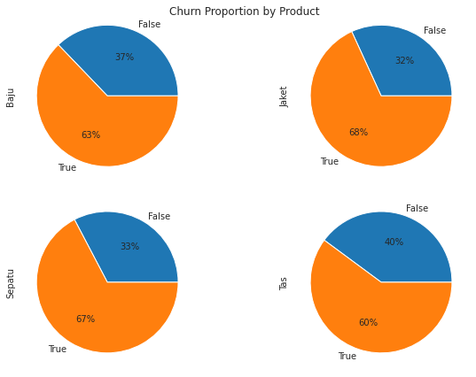
Churn Customer Proportion
# Create pivot table
churn_prop = df.pivot_table(index='is_Churn',
                        columns='Product',
                        values='Customer_ID',
                        aggfunc='count',
                        fill_value=0)
churn_prop
| Product | Baju | Jaket | Sepatu | Tas |
|---|---|---|---|---|
| is_Churn | ||||
| False | 1268 | 11123 | 16064 | 4976 |
| True | 2144 | 23827 | 33090 | 7508 |
# Plotting churn proportion using pie plot
churn_prop.plot.pie(subplots=True, layout=(2,2), autopct='%1.0f%%',
                    legend=False, title='Churn Proportion by Product')
plt.tight_layout()
Distribution Count Transaction
# Create function distribution count transaction
def distribution_count_trans(row):
    if row['Count_Transaction'] == 1:
        val = '1'
    elif (row['Count_Transaction'] > 1 and row['Count_Transaction'] <= 3):
        val ='2 - 3'
    elif (row['Count_Transaction'] > 3 and row['Count_Transaction'] <= 6):
        val ='4 - 6'
    elif (row['Count_Transaction'] > 6 and row['Count_Transaction'] <= 10):
        val ='7 - 10'
    else:
        val ='> 10'
    return val
# Apply function to new column
df['Count_Transaction_Group'] = df.apply(distribution_count_trans, axis=1)
# Grouping Number of Customers by Count Transaaction Group
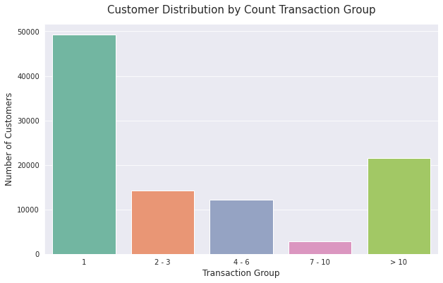
count_trans_group = df.groupby(['Count_Transaction_Group'])['Customer_ID'].count()
count_trans_group
Count_Transaction_Group
1         49255
2 - 3     14272
4 - 6     12126
7 - 10     2890
> 10      21457
Name: Customer_ID, dtype: int64
# Plotting count transaction group
sns.barplot(x = count_trans_group.index, y = count_trans_group, palette='Set2')
plt.title('Customer Distribution by Count Transaction Group', fontsize=15, pad=15)
plt.xlabel('Transaction Group', fontsize=12)
plt.ylabel('Number of Customers', fontsize=12)
Text(0, 0.5, 'Number of Customers')
Distribution Average Transaction
# Create function distribution average transaction
def distribution_avg_trans(row):
    if (row['Average_Transaction_Amount'] >= 100000 and row['Average_Transaction_Amount'] <= 200000):
        val ='100.000 - 250.000'
    elif (row['Average_Transaction_Amount'] > 250000 and row['Average_Transaction_Amount'] <= 500000):
        val ='>250.000 - 500.000'
    elif (row['Average_Transaction_Amount'] > 500000 and row['Average_Transaction_Amount'] <= 750000):
        val ='>500.000 - 750.000'
    elif (row['Average_Transaction_Amount'] > 750000 and row['Average_Transaction_Amount'] <= 1000000):
        val ='>750.000 - 1.000.000'
    elif (row['Average_Transaction_Amount'] > 1000000 and row['Average_Transaction_Amount'] <= 2500000):
        val ='>1.000.000 - 2.500.000'
    elif (row['Average_Transaction_Amount'] > 2500000 and row['Average_Transaction_Amount'] <= 5000000):
        val ='>2.500.000 - 5.000.000'
    elif (row['Average_Transaction_Amount'] > 5000000 and row['Average_Transaction_Amount'] <= 10000000):
        val ='>5.000.000 - 10.000.000'
    else:
        val ='>10.000.000'
    return val
# Apply function to new column
df['Average_Transaction_Amount_Group'] = df.apply(distribution_avg_trans, axis=1)
# Grouping Number of Customers by Average Transaction Amount Group
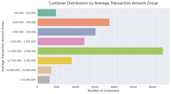
avg_trans_group = df.groupby(['Average_Transaction_Amount_Group'])['Customer_ID'].count()
avg_trans_group
Average_Transaction_Amount_Group
100.000 - 250.000           4912
>1.000.000 - 2.500.000     32819
>10.000.000                 3227
>2.500.000 - 5.000.000      9027
>250.000 - 500.000         18857
>5.000.000 - 10.000.000     3689
>500.000 - 750.000         15171
>750.000 - 1.000.000       12298
Name: Customer_ID, dtype: int64
# Plotting average transaction amount group
orders = ['100.000 - 250.000', '>250.000 - 500.000', '>500.000 - 750.000',
          '>750.000 - 1.000.000', '>1.000.000 - 2.500.000', '>2.500.000 - 5.000.000',
          '>5.000.000 - 10.000.000', '>10.000.000']
sns.barplot(x = avg_trans_group, y = avg_trans_group.index, order=orders, palette='Set2')
plt.title('Customer Distribution by Average Transaction Amount Group', fontsize=15, pad=15)
plt.xlabel('Number of Customers', fontsize=12)
plt.ylabel('Average Transaction Amount Group', fontsize=12)
Text(0, 0.5, 'Average Transaction Amount Group')
Data Modelling
Feature Engineering
# Check datatypes
df.dtypes
Customer_ID                                  int64
Product                                     object
First_Transaction                   datetime64[ns]
Last_Transaction                    datetime64[ns]
Average_Transaction_Amount                   int64
Count_Transaction                            int64
is_Churn                                    object
Year_First_Transaction                       int64
Year_Last_Transaction                        int64
Count_Transaction_Group                     object
Average_Transaction_Amount_Group            object
dtype: object
# Copy old dataframe
df_model = df.copy()
# Create new column from First Transaction
df_model['Month_First'] = df_model['First_Transaction'].dt.month
df_model['Day_First'] = df_model['First_Transaction'].dt.day
# Create new column from Last Transaction
df_model['Month_Last'] = df_model['Last_Transaction'].dt.month
df_model['Day_Last'] = df_model['Last_Transaction'].dt.day
# Encoding categorical data
df_model['Count_Transaction_Group'].replace({'1':0, '2 - 3':1, '4 - 6':2, '7 - 10':3,
                                             '> 10':4}, inplace=True)
amounts = {'100.000 - 250.000':0, '>250.000 - 500.000':1, '>500.000 - 750.000':2,
          '>750.000 - 1.000.000':3, '>1.000.000 - 2.500.000':4, '>2.500.000 - 5.000.000':5,
          '>5.000.000 - 10.000.000':6, '>10.000.000':7}
df_model['Average_Transaction_Amount_Group'].replace(amounts, inplace=True)
df_model['is_Churn'].replace({False:0, True:1}, inplace=True)
# Perform one hot encoding
df_encode = pd.get_dummies(df_model['Product'])
# Selected columns
remove_cols = ['Product', 'First_Transaction', 'Last_Transaction', 'Count_Transaction', 'Average_Transaction_Amount']
df_fix = df_model.drop(remove_cols, axis=1)
# Concatenate dataframe
df_model_fix = pd.concat([df_fix, df_encode], axis=1)

# Check new first five rows
df_model_fix.head()
| Customer_ID | is_Churn | Year_First_Transaction | Year_Last_Transaction | Count_Transaction_Group | Average_Transaction_Amount_Group | Month_First | Day_First | Month_Last | Day_Last | Baju | Jaket | Sepatu | Tas | |
|---|---|---|---|---|---|---|---|---|---|---|---|---|---|---|
| 0 | 29531 | 0 | 2016 | 2018 | 4 | 4 | 6 | 19 | 10 | 5 | 0 | 1 | 0 | 0 |
| 1 | 29531 | 0 | 2014 | 2018 | 4 | 4 | 7 | 23 | 12 | 25 | 0 | 0 | 1 | 0 |
| 2 | 141526 | 0 | 2017 | 2019 | 4 | 1 | 4 | 28 | 1 | 24 | 0 | 0 | 0 | 1 |
| 3 | 141526 | 0 | 2017 | 2019 | 4 | 2 | 4 | 28 | 1 | 16 | 0 | 1 | 0 | 0 |
| 4 | 37545 | 0 | 2015 | 2018 | 4 | 4 | 4 | 16 | 11 | 22 | 0 | 0 | 1 | 0 |
# Check new data type
df_model_fix.dtypes
Customer_ID                         int64
is_Churn                            int64
Year_First_Transaction              int64
Year_Last_Transaction               int64
Count_Transaction_Group             int64
Average_Transaction_Amount_Group    int64
Month_First                         int64
Day_First                           int64
Month_Last                          int64
Day_Last                            int64
Baju                                uint8
Jaket                               uint8
Sepatu                              uint8
Tas                                 uint8
dtype: object
# View Total Proportion Churn
df_model_fix['is_Churn'].value_counts(normalize=True)
1    0.66569
0    0.33431
Name: is_Churn, dtype: float64
Split Train and Test Data
# Choose feature columns
X = df_model_fix.drop(['is_Churn'], axis=1)
# Choose target columns
y = df_model_fix['is_Churn']

# Split train and test set
X_train, X_test, y_train, y_test = train_test_split(X, y, test_size=0.25, random_state=42)
Model Selection
# Create function choose model
def choose_model(model_name):
  # Train model
  model = model_name.fit(X_train, y_train)
  # Scoring Model
  model_score = model.score(X_test, y_test)
  print(f'Score Accuracy is {round(model_score*100, 2)}%')
  # Validating Model
  valid_score = np.mean(cross_val_score(model_name, X_train, y_train, cv=5))
  print(f'Score Validation is {round(valid_score*100, 2)}%')
# Choose model
choose_model(LogisticRegression())
Score Accuracy is 72.19%
Score Validation is 74.93%
# Choose model
choose_model(xgb.XGBClassifier())
Score Accuracy is 100.0%
Score Validation is 100.0%
Model Evaluation
# Function for plot confusion matrix and classification report
def check_matrix_and_reports(model_plot):
  # Churn Prediction
  train = model_plot.fit(X_train, y_train)
  preds = train.predict(X_test)

  # Create confusion matrix
  class_names = ['Not Churn', 'Churn']
  cnf_matrix = confusion_matrix(y_test, preds)
  # Use subplotting
  fig, ax = plt.subplots(figsize=(8,4))
  tick_marks = np.arange(len(class_names))
  plt.xticks(tick_marks, class_names)
  plt.yticks(tick_marks, class_names)
  # Plotting using heatmap
  sns.heatmap(pd.DataFrame(cnf_matrix), annot=True, cmap='YlGnBu', fmt='g')
  plt.title('Confusion matrix', fontsize=15, pad=15)
  plt.xlabel('Actual')
  plt.ylabel('Predicted')

  # Create classification report
  reports = classification_report(y_test, preds, target_names=class_names)
  print('Classification Report\n', reports)
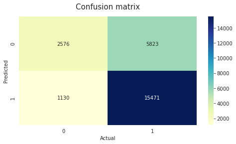
# Apply function with Logistic Regression
check_matrix_and_reports(LogisticRegression())
Classification Report
               precision    recall  f1-score   support

   Not Churn       0.70      0.31      0.43      8399
       Churn       0.73      0.93      0.82     16601

    accuracy                           0.72     25000
   macro avg       0.71      0.62      0.62     25000
weighted avg       0.72      0.72      0.69     25000
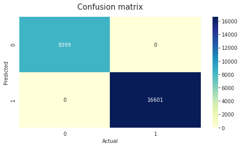
# Apply function with XGBoost Classifier
check_matrix_and_reports(xgb.XGBClassifier())
Classification Report
               precision    recall  f1-score   support

   Not Churn       1.00      1.00      1.00      8399
       Churn       1.00      1.00      1.00     16601

    accuracy                           1.00     25000
   macro avg       1.00      1.00      1.00     25000
weighted avg       1.00      1.00      1.00     25000
# Predict probability of churn
model1 = LogisticRegression().fit(X_train, y_train)
log_pred = model1.predict_proba(X_test)[:,1]
model2 = xgb.XGBClassifier().fit(X_train, y_train)
xgb_pred = model2.predict_proba(X_test)[:,1]

# ROC Chart components
fallout_log, sensitivity_log, thresholds_log = roc_curve(y_test, log_pred)
fallout_xgb, sensitivity_xgb, thresholds_xgb = roc_curve(y_test, xgb_pred)

# ROC Chart with both
plt.plot(fallout_log, sensitivity_log, color = 'blue', label='%s' % 'Logistic Regression')
plt.plot(fallout_xgb, sensitivity_xgb, color = 'green', label='%s' % 'XGBoost')
plt.plot([0, 1], [0, 1], linestyle='--', label='%s' % 'Random Prediction')
plt.title("ROC Chart on Probability of Churn")
plt.xlabel('Fall-out')
plt.ylabel('Sensitivity')
plt.legend()
<matplotlib.legend.Legend at 0x7f2d2a3b0f90>
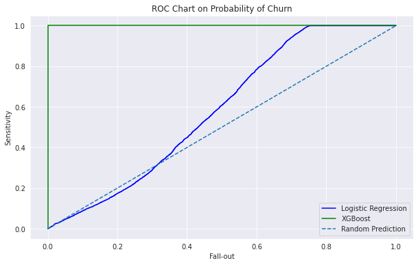
# Print the logistic regression AUC with formatting
print("Logistic Regression AUC Score: %0.2f" % roc_auc_score(y_test, log_pred))

# Print the xgboost classifier AUC with formatting
print("XGBoost Classifier AUC Score: %0.2f" % roc_auc_score(y_test, xgb_pred))
Logistic Regression AUC Score: 0.58
XGBoost Classifier AUC Score: 1.00